Mapping life satisfaction with Leaflet in R
It wasn’t until after I went through the whole process of using Leaflet.js that I discovered that there is a Leaflet package for R!. The documentation promised that “this R package makes it easy to integrate and control Leaflet maps in R”, and they weren’t wrong.
To test it out, I got a hold of some data on life satisfaction by borough, sourced from the Annual Population Survey (APS) Well-being dataset. The data is organised by borough, and I chose the metric of ‘general life satisfaction’. Participants were asked, “Overall, how satisfied are you with your life right now”, and asked to nominate a score between 0 (“not at all”), and 10 (“completely”). The shapefiles were sourced from the London Datastore.
Here’s how the final map ended up:
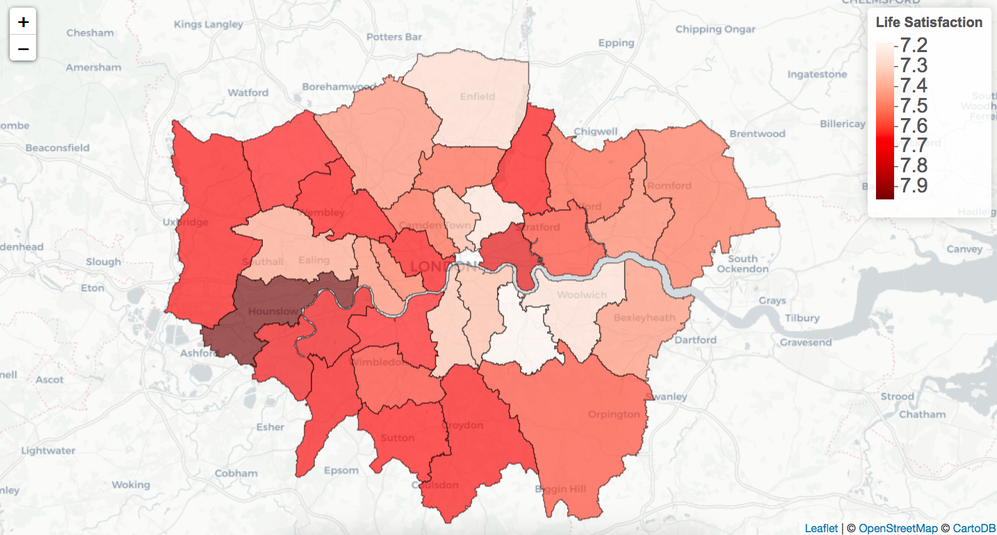
(Looks like Hounslow is the place to be. Lewisham…not so much.)
And here’s the full code:
library(readxl)
library(tidyverse)
library(skimr)
library(leaflet)
library(sp)
library(rgdal)

##Read in the data

mydata <- read_xls("~/Downloads/personal-well-being-borough.xls", sheet=2)

##Light editing of data

mydata <- mydata[4:35, c(2,8)]
colnames(mydata) <- c("NAME","Life_Satisfaction")
mydata$Life_Satisfaction <- as.numeric(mydata$Life_Satisfaction)

##Read in the spatial data

setwd("~/Downloads/statistical-gis-boundaries-london/ESRI")
boroughs <- readOGR(dsn = ".")

##Merge with boroughs

boroughs <- merge(boroughs, mydata, by = "NAME")

##Transform the data to appropriate coordinate system
boroughs <- spTransform(boroughs, CRS("+init=epsg:4326"))

#Filter out City of London - no data
boroughs <- boroughs[boroughs$NAME!="City of London", ]

##Define the colour palette
pal <- colorNumeric(palette = "Reds", domain = boroughs$Life_Satisfaction)

##Map
leaflet() %>%
  addProviderTiles("CartoDB.Positron", options= providerTileOptions(opacity = 0.99)) %>%
  addPolygons(data = boroughs, stroke = TRUE, color="black", weight=1, fillOpacity = 0.65,
              smoothFactor = 0.5, fillColor = ~pal(Life_Satisfaction)) %>%
  addLegend(pal = pal, values = ~Life_Satisfaction,
            opacity=1, title = "Life Satisfaction")
A few things to note:
- The
spTransformfunction is used to transform the data to an appropriate projected coordinate system; - You can’t use the tidyverse pipe with sp objects, so I filtered the borough data ‘the base way’ (using susetting rather than dplyr’s ‘filter’ function)
- Colour is mapped separately, in this case by assigning to
pal